Random Sample Imputation

Till now we have seen techniques that were either applicable for Numerical or Categorical variables but not both. So we would like to make you familiar with a new technique that can be easily used for both the Numerical & Categorical variables.  

Random Sample Imputation is the technique that is widely used for both the Numerical and Categorical Variables. Do not confuse it with Arbitrary Value Imputation, may seems to be similar by name. In fact, it's totally different.

When compared based on the principle used for imputation, it is more similar to Mean/Median/Mode Imputation techniques. This technique also preserves the statistical parameter of the original variable distribution, for the missing data just like Mean/Median/Mode Imputations.

Now let's go ahead and have a look at the assumptions that we need to keep in mind, advantages and the limitations of this technique, post that we will be getting our hands dirty with some code.

Key Points to Remember

This Imputation technique can be used for both the Numerical and Categorical variables.

The process of Random Sampling involves replacing the missing values by taking a random observation from the pool of available observations for the variable. 

Here, we have not limited to only one(1) Random observation, rather take as many random observations as the number of missing values for the variable.

Thus, by doing so we can ensure that the mean and standard deviation of the variables is not changed (preserved) for Numerical variables. Whereas for the Categorical variable, the frequency of the categories is preserved(not changed).

Another thing we can keep a note of here is that, since the variable distribution is preserved, we can use this method for Linear models.

To use this method for Missing Data At Random, we need to use a missing data indicator in combination with this technique.

Assumptions

• The data is Missing Completely At Random(MCAR).
• We replace the missing values with the values having the same distribution of original variables.
• The probability of selecting the value is dependent on its frequency, i.e. higher the frequency of a value higher the probability of selecting it. Thus, the variance & distribution of variables is preserved.
• Missing values are not more than 5% of the complete dataset.

Advantages

• It is easy to implement.
• We can get the complete dataset very quickly.
• The variance & distribution of variables is preserved.

Limitations

• Randomness -- Since the value of missing data is selected at random, there is always a chance of getting different values for the same observation. This can be controlled by using "seed" during the process.
• In case we have more missing values, then the relationship of the imputed variable with other variables may be affected.
• For extracting the values for Test Set we need to store the train set in memory, as the missing values should always be replaced by the values of the Train set only. Thus, in the case of huge data sets, it becomes a memory-intensive operation.

Code

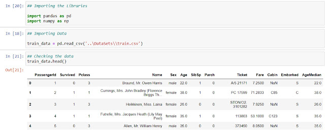
1. Importing the Libraries and the data.

Importing the Libraries and the data.

2. Let's check the percentage of missing values in each column.

check the percentage of missing values

3. Copying the data in a new column and pre-processing.

Here, we will first create a new variable "Age_Imputed", so that our original variable is not disturbed. 

 

Create a new variable "Age_Imputed"

Now, we need to find the random values from the data and the index of missing values for replacement. 
We will be storing this value in a new variable "random_sample_train". 

We are using a random state of "18" to avoid randomness. 

Finding Random Values

4. Performing Imputation

We will be using the values from "random_sample_train" for imputation. 

Performing Imputation

Now, time to verify if the Imputation has been performed or not.

Verifying Imputation

5. Verifying Imputation

Let's have a look at the values that are imputed. 

Verifying Imputation

We can see here that 3 different values have been imputed for 3 different missing values.

Now, as said that this method preserves the variance, time to verify it. 

Verifying Variance

There are many Python libraries also which we can use and perform the Random Sample Imputation directly in a single line of code. We will be covering that part in a separate article.

Summary

In this Quick Note, we studied a famous Imputation Technique, i.e. Random Sample Imputation. We looked at the assumptions, advantages and disadvantages of the method and also basic coding in python to achieve Random Sample Imputation. 

That's all from Here. Until Then... This is Quick Data Science Team signing off.

Comment below to get the complete notebook and dataset.