Discretisation -- Equal Frequency

 

We have studied a few techniques commonly used for the process of Discretisation or binning. We are here to discuss another important technique that we can use for binning is -- dividing the data into equal size groups, i.e. total data is divided into groups/bins each containing an equal amount of data. 

The important part here to note is that widths of each bin may defer in this case, i.e. one bin can be 0-5 and another might be of size 70-100. 

Example

Let's have an example to understand the whole thing better. 

We would be using the same old "Age column from Tiatianic Dataset" to understand this concept. 

Age Distribution

The above graph shows the normal distribution of the 'Age' variable in the titanic data, We could notice that there is a high concentration of observations in the middle but very little at both ends. 

Thus, to remove this skewness from our data, what we can do is, we can bundle the data together in approximately equal size such that each bin/group has an equal say in the graph and data looks more organised and analysable. 

 

When to Use?

Now, the next that comes to our mind is, When we can use it?

So, basically, this technique is used when the data is highly skewed, i.e. has more concentration at any of the ends. As the sole purpose of this technique is to distribute the data evenly across the bins. 

How to Use?

Another common issue that we face here is How to decide the size of each bin? i.e. How many values should be assigned to a bin. 

Do not Worry... This is simple, we need to divide the data into Quantiles(Q1, Q2, Q4 & so on...). Once we have decided the number of quantiles we want for our data, the rest of the thing becomes simple.

Practical

We will be using the feature-engine library of python for demo purposes.

1. Importing the Libraries

Importing Equal Frequency Discretiser, libraries and data

2. Data Visualization

Since, we will be using only "Age" column of the data set for Discretisation, let's see how it looks when we visualise it. 

Data Visuals before Binning

We already discussed this graph above in example.

3. Using the Equal Frequency Discretiser

Initializing the Equal Frequency Discretiser

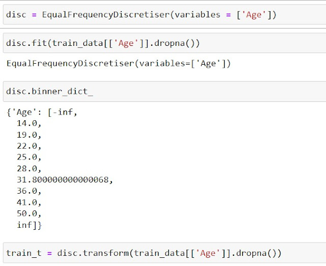
In first line we have initialized the Equal Frequency Discretiser, then used to fit it on "Age" column.

Once we are done with it, using the "binner_dict_" function we can see that the function has created bins automatically. 

4. Visualizing the End Result

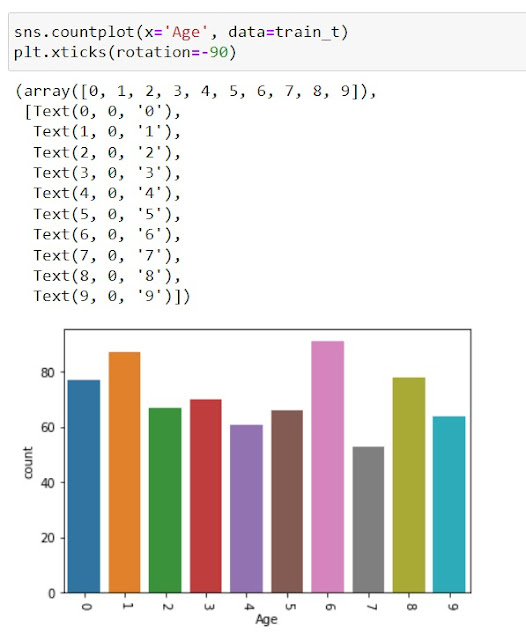
Equal Frequency Discretisation Result

We could notice here that the shape of the original graph is not retained in the final result, i.e. higher values in middle, least on the right end. We have re-distributed the values in these 10 bins such that each bin has approximately equal values.

Resources

Please comment below to get the complete dataset and libraries. 

Learn to install Anaconda Here.

Learn about the Feature-Engine library Here.

Summary 

In this Quick Reads, we studied a technique, Equal Frequency Discretisation that is commonly used for Discretisation. We had a quick overview of the technique, understood how and why to use it and some quick Points to Remember. 

We also performed a practical demo of this technique using a famous python library "feature-engine". 

 Last but not least... "Practice Makes One Perfect". So what are you waiting for practice this technique and comment below your views, doubts or anything? We are here to help you.